Discounted Return

0<= 𝞬 <=1
the agent will only care about if immediate rewards if 𝞬 = 0
the agent will care more about future rewards if 𝞬 is large

Epsilon-Greedy Policies

0<= ε <=1
the agent selects the greedy action with probability 1- ε
the agent selects an action uniform at random from the set of available(non-greedy AND greedy) actions with probability ε
so if ε = 0, the agent always select the greedy action

Constant-alpha

0<= 𝛼 <=1
If 𝛼 = 0, then the action-value function estimate is never updated by the agent.
If 𝛼 = 1, then the final value estimate for each state-action pair is always equal to the last return that was experienced by the agent (after visiting the pair).
Smaller values for 𝛼 encourage the agent to consider a longer history of returns when calculating the action-value function estimate.
Increasing the value of 𝛼 ensures that the agent focuses more on the most recently sampled returns.
When implementing constant-𝛼 MC control, you must be careful to not set the value of git α too close to 1.
This is because very large values can keep the algorithm from converging to the optimal policy 𝛑∗.
However, you must also be careful to not set the value of 𝛼 too low, as this can result in an agent who learns too slowly.
The best value of 𝛼 for your implementation will greatly depend on your environment and is best gauged through trial-and-error.

Reading Scientific Papers

As part of this nanodegree, you will learn about many of the most recent, cutting-edge algorithms! Because of this, it will prove useful to learn how to read the original research papers. Here are some excellent tips. Some of the best advice is:

• Take notes.
• Read the paper multiple times. On the first couple readings, try to focus on the main points:
  1. What kind of tasks are the authors using deep reinforcement learning (RL) to solve? What are the states, actions, and rewards?
  2. What neural network architecture is used to approximate the action-value function?
  3. How are experience replay and fixed Q-targets used to stabilize the learning algorithm?
  4. What are the results?
• Understanding the paper will probably take you longer than you think. Be patient, and reach out to the Udacity community with any questions.

pre-processing steps for FashionMNIST data creation

Best practice to place layers

Best practice is to place any layers whose weights will change during the training process in init and refer to them in the forward function; any layers or functions that always behave in the same way, such as a pre-defined activation function, may appear in the init or in the forward function; it is mostly a matter of style and readability.

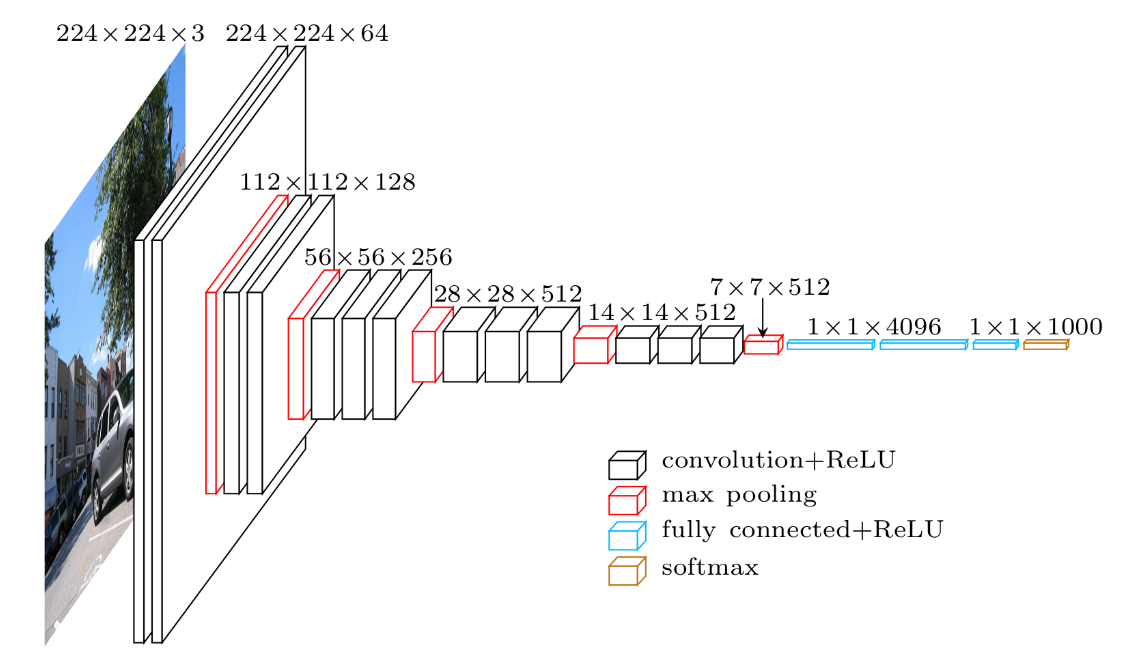
VGG-16 architecture

Clasisification vs. Regression

The loss function you should choose depends on the kind of CNN you are trying to create; cross entropy is generally good for classification tasks, but you might choose a different loss function for, say, a regression problem that tried to predict (x,y) locations for the center or edges of clothing items instead of class scores.

Cnn output size

For any convolutional layer, the output feature maps will have the specified depth (a depth of 10 for 10 filters in a convolutional layer) and the dimensions of the produced feature maps (width/height) can be computed as the input image width/height, W, minus the filter size, F, divided by the stride, S, all + 1. The equation looks like: output_dim = (W-F)/S + 1, for an assumed padding size of 0. You can find a derivation of this formula, here.
For a pool layer with a size 2 and stride 2, the output dimension will be reduced by a factor of 2. Read the comments in the code below to see the output size for each layer.

Policy-Based Methods Study plan(for review in future)

Lesson: Introduction to Policy-Based Methods

In this lesson, you will learn about methods such as hill climbing, simulated annealing, and adaptive noise scaling. You’ll also learn about cross-entropy methods and evolution strategies.

Lesson: Policy Gradient Methods

In this lesson, you’ll study REINFORCE, along with improvements we can make to lower the variance of policy gradient algorithms.

Lesson: Proximal Policy Optimization

In this lesson, you’ll learn about Proximal Policy Optimization (PPO), a cutting-edge policy gradient method.

Lesson: Actor-Critic Methods

In this lesson, you’ll learn how to combine value-based and policy-based methods, bringing together the best of both worlds, to solve challenging reinforcement learning problems.

Lesson: Deep RL for Finance (Optional)

In this optional lesson, you’ll learn how to apply deep reinforcement learning techniques for optimal execution of portfolio transactions.

Resources (Optional)

• Read the most famous blog post on policy gradient methods.
• Implement a policy gradient method to win at Pong in this Medium post.
• Learn more about evolution strategies from OpenAI.

Value-based Methods vs Policy-based Methods

• With value-based methods, the agent uses its experience with the environment to maintain an estimate of the optimal action-value function. The optimal policy is then obtained from the optimal action-value function estimate.
• Policy-based methods directly learn the optimal policy, without having to maintain a separate value function estimate.

Policy Function Approximation

• In deep reinforcement learning, it is common to represent the policy with a neural network.
  • This network takes the environment state as input.
  • If the environment has discrete actions, the output layer has a node for each possible action and contains the probability that the agent should select each possible action.
• The weights in this neural network are initially set to random values. Then, the agent updates the weights as it interacts with (and learns more about) the environment.

More on the Policy

• Policy-based methods can learn either stochastic or deterministic policies, and they can be used to solve environments with either finite or continuous action spaces.

Hill Climbing

• Hill climbing is an iterative algorithm that can be used to find the weights \thetaθ for an optimal policy.
• At each iteration,
  • We slightly perturb the values of the current best estimate for the weights \theta_{best}θ best, to yield a new set of weights.
  • These new weights are then used to collect an episode. If the new weights \theta_{new}θ new resulted in higher return than the old weights, then we set \theta_{best} \leftarrow \theta_{new}θ best ←θ new.

Beyond Hill Climbing

• Steepest ascent hill climbing is a variation of hill climbing that chooses a small number of neighboring policies at each iteration and chooses the best among them.
• Simulated annealing uses a pre-defined schedule to control how the policy space is explored, and gradually reduces the search radius as we get closer to the optimal solution.
• Adaptive noise scaling decreases the search radius with each iteration when a new best policy is found, and otherwise increases the search radius.

More Black-Box Optimization

• The cross-entropy method iteratively suggests a small number of neighboring policies, and uses a small percentage of the best performing policies to calculate a new estimate.
• The evolution strategies technique considers the return corresponding to each candidate policy. The policy estimate at the next iteration is a weighted sum of all of the candidate policies, where policies that got higher return are given higher weight.

Why Policy-Based Methods?

There are three reasons why we consider policy-based methods:

• Simplicity: Policy-based methods directly get to the problem at hand (estimating the optimal policy), without having to store a bunch of additional data (i.e., the action values) that may not be useful.
• Stochastic policies: Unlike value-based methods, policy-based methods can learn true stochastic policies.
• Continuous action spaces: Policy-based methods are well-suited for continuous action spaces.

Policy Gradient Methods Why We use Trajectories?

You may be wondering: why are we using trajectories instead of episodes? The answer is that maximizing expected return over trajectories (instead of episodes) lets us search for optimal policies for both episodic and continuing tasks!

That said, for many episodic tasks, it often makes sense to just use the full episode. In particular, for the case of the video game example described in the lessons, reward is only delivered at the end of the episode. In this case, in order to estimate the expected return, the trajectory should correspond to the full episode; otherwise, we don’t have enough reward information to meaningfully estimate the expected return.

An overview of gradient descent optimization algorithms

optimizing gradient descent

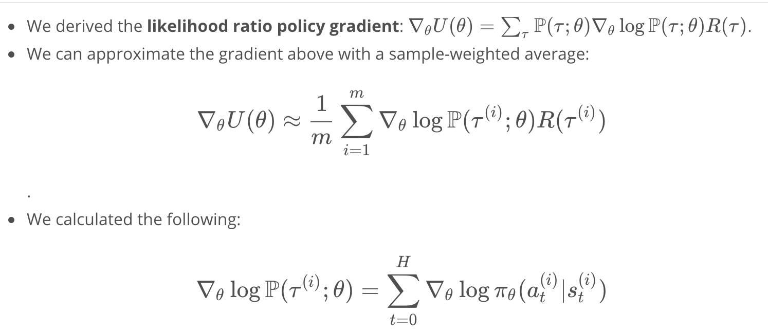
Likelihood ratio policy gradient

etc…

evolution-strategies

We’ve discovered that evolution strategies (ES), an optimization technique that’s been known for decades, rivals the performance of standard reinforcement learning (RL) techniques on modern RL benchmarks (e.g. Atari/MuJoCo), while overcoming many of RL’s inconveniences

What are Policy Gradient Methods?

• Policy-based methods are a class of algorithms that search directly for the optimal policy, without simultaneously maintaining value function estimates.
• Policy gradient methods are a subclass of policy-based methods that estimate the weights of an optimal policy through gradient ascent.
• In this lesson, we represent the policy with a neural network, where our goal is to find the weights \thetaθ of the network that maximize expected return.

The Big Picture Of Policy Gradient Method

The policy gradient method will iteratively amend the policy network weights to:

• make (state, action) pairs that resulted in positive return more likely, and
• make (state, action) pairs that resulted in negative return less likely.

Policy Gradient Method Problem Setup

• A trajectory τ is a state-action sequence s_0, a_0, s, s_H, a_H, s_{H+1}
• In this lesson, we will use the notation R(τ) to refer to the return corresponding to trajectory τ
• Our goal is to find the weights θ of the policy network to maximize the expected return

Policy Gradient Reinforce

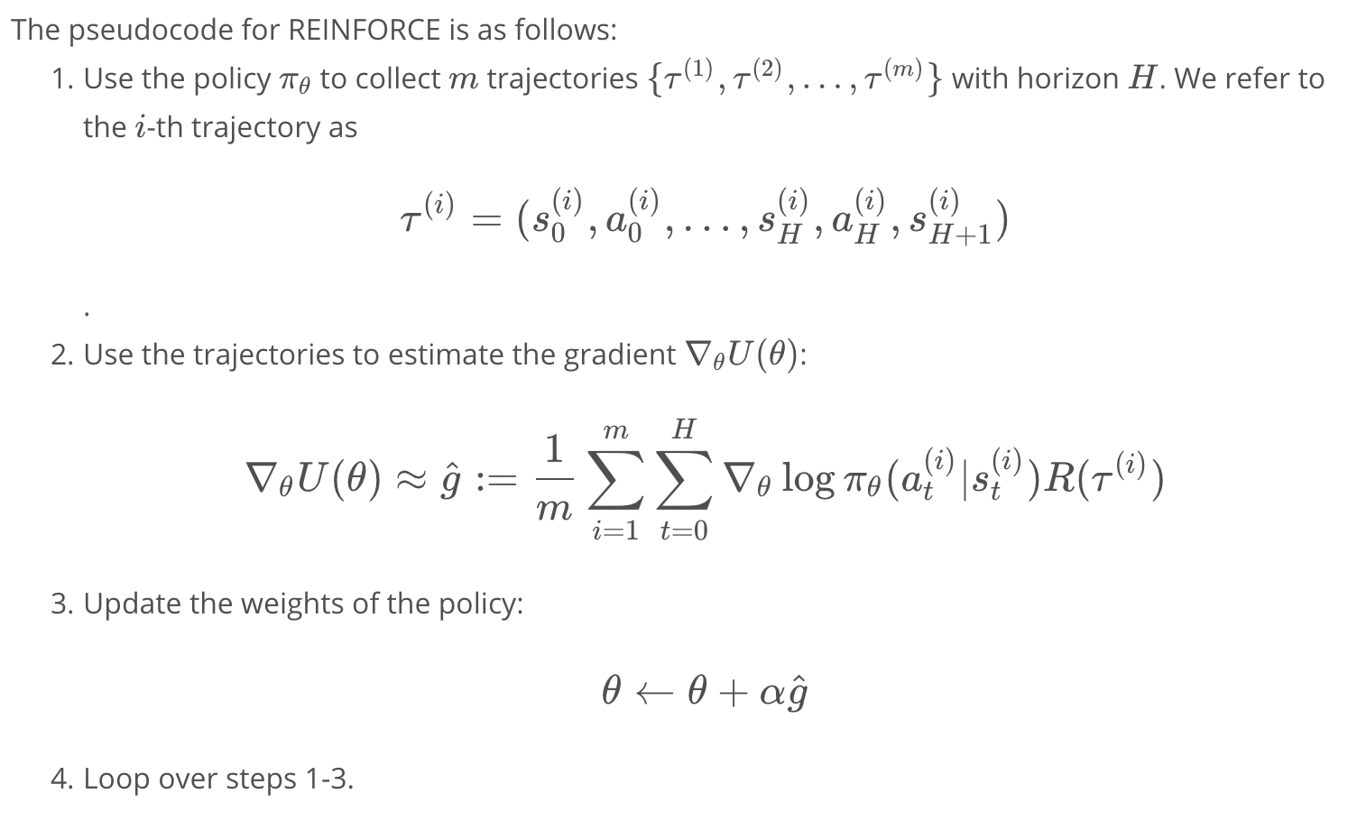
Policy Gradient Derivation

Proximal Policy Optimization (PPO)

link

Notes on Gradient Modification

Notes on Gradient Modification You might wonder, why is it okay to just change our gradient? Wouldn’t that change our original goal of maximizing the expected reward?

It turns out that mathematically, ignoring past rewards might change the gradient for each specific trajectory, but it doesn’t change the averaged gradient. So even though the gradient is different during training, on average we are still maximizing the average reward. In fact, the resultant gradient is less noisy, so training using future reward should speed things up!

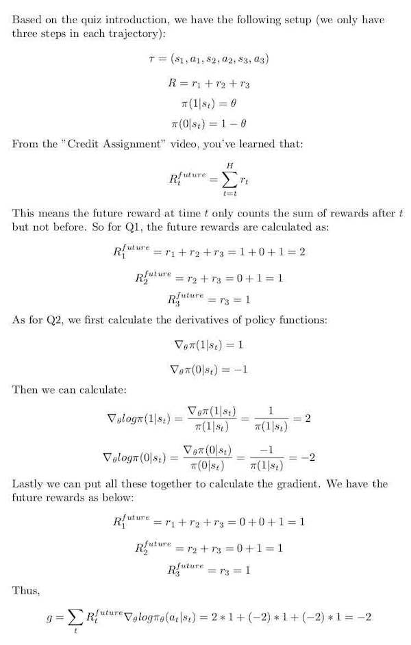
Policy Gradient Quiz Equation

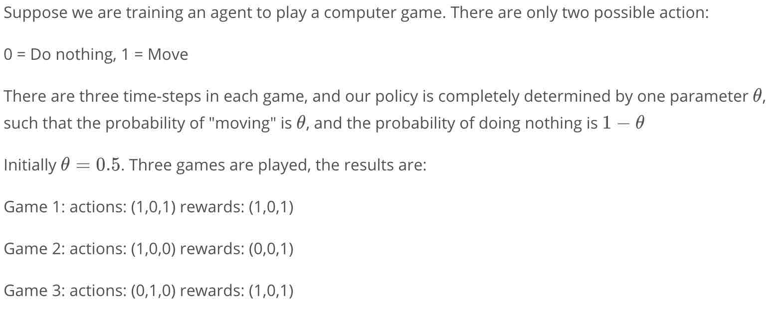
For a better formatted version of the explanation below, please check explanation

Pong with REINFORCE (code walkthrough)

• The performance for the REINFORCE version may be poor. You can try training with a smaller tmax=100 and more number of episodes=2000 to see concrete results.
• Try normalizing your future rewards over all the parallel agents, it can speed up training
• Simpler networks might perform better than more complicated ones! The original input contains 80x80x2=12800 numbers, you might want to ensure that this number steadily decreases at each layer of the neural net.
• Training performance may be significantly worse on local machines. I had worse performance training on my own windows desktop with a 4-core CPU and a GPU. This may be due to the slightly different ways the emulator is rendered. So please run the code on the workspace first before moving locally
• It may be beneficial to train multiple epochs, say first using a small tmax=200 with 500 episodes, and then train again with tmax = 400 with 500 episodes, and then finally with a even larger tmax.
• Remember to save your policy after training!
• for a challenge, try the ‘Pong-v4’ environment, this includes random frameskips and takes longer to train.

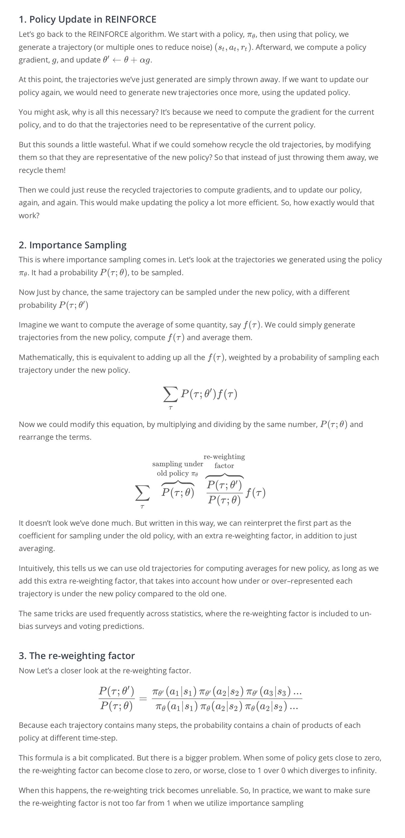
  Importance Sampling

  

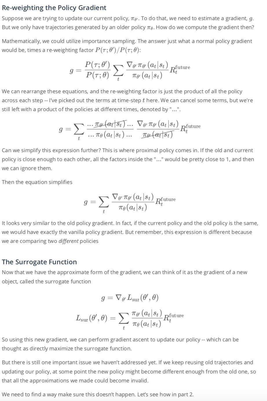
  The Surrogate Function

  

  Clipping Policy Updates

  

  PPO Summary

  more detail